by Arup Nanda
Part 5 of a five-part series that presents an easier way to learn Python by comparing and contrasting it to PL/SQL.
Python with Data and Oracle Database
I hope you have enjoyed learning about Python as the complexity developed progressively in this series until this point. So far, we have covered the elements of the language and how you use them in place of PL/SQL programs you are already familiar with. But since you are most likely a PL/SQL developer, you are a data professional by trade. Your objective, it can be argued, is to manipulate data—in fact large amounts of it. Can you use Python for that? Of course you can.
Earlier you saw some examples of native data handling capabilities of Python expressed in collections (lists, tuples, dictionaries, and so on) that can store large amounts of data in memory and manipulate them well. But, there is more: much, much more. Python offers built-in modules for advanced data handling and visualization to turn data into knowledge, which is the essence of data science.
In this installment you will learn about these data manipulation modules, specifically NumPy, Pandas, MatPlotLib, SQL Alchemy, and CX_Oracle. The last two are for Python programs to connect to Oracle Database, similar to Pro*C.
A word to set expectations may be prudent here: each of these modules is vast enough to cover in a book, let alone a few sections in an article. It's not my intention to present this installment of the series as a complete treatise of these topics. Rather it's an attempt to jumpstart the learning process by providing just the right amount of information. Once you master the basics, you will find much easier to explore the subjects with the help of the documentation.
Installation
All the Python modules are not installed by default. They may need to be installed explicitly after Python is installed. The simplest way to install the modules is to use the Python Installer Package (PIP), which is somewhat similar to what an app store is to a smartphone. To learn what modules are available for extending Python, simply visit the Python Package Index (PyPI) index page. You can invoke the PIP to install the appropriate module.
Here is how you install a module named oracle-db-query. Please note that oracle-db-query is not discussed in this article. It's merely shown here as an example of how to install a package.
C:\>python -m pip install oracle-db-query
Collecting oracle-db-query
Downloading oracle_db_query-1.0.0-py3-none-any.whl
Collecting pyaml (from oracle-db-query)
Downloading pyaml-15.8.2.tar.gz
Requirement already satisfied (use --upgrade to upgrade): pandas in c:\python34\lib\site-packages (from oracle-db-query)
Requirement already satisfied (use --upgrade to upgrade):
cx-Oracle in
c:\python34\lib\site-packages\cx_oracle-5.2.1-py34-win32.egg (from
oracle-db-query)
Collecting PyYAML (from pyaml->oracle-db-query)
Downloading PyYAML-3.11.zip (371kB)
100% |################################| 378kB 2.2MB/s
Requirement already satisfied (use --upgrade to upgrade):
numpy>=1.7.0 in c:\python34\lib\site-packages (from
pandas->oracle-db-query)
Requirement already satisfied (use --upgrade to upgrade):
python-dateutil>=2 in c:\python34\lib\site-packages (from
pandas->oracle-db-query)
Requirement already satisfied (use --upgrade to upgrade):
pytz>=2011k in c:\python34\lib\site-packages (from
pandas->oracle-db-query)
Requirement already satisfied (use --upgrade to upgrade):
six>=1.5 in c:\python34\lib\site-packages (from
python-dateutil>=2->pandas->oracle-db-query)
Building wheels for collected packages: pyaml, PyYAML
Running setup.py bdist_wheel for pyaml ... done
Stored in directory:
C:\Users\arupnan\AppData\Local\pip\Cache\wheels\b3\a1\20\62a3bb21201ef3d01e1f41ca396871750998bc00e6697f992d
Running setup.py bdist_wheel for PyYAML ... done
Stored in directory:
C:\Users\arupnan\AppData\Local\pip\Cache\wheels\4a\bf\14\d79994d19a59d4f73efdafb8682961f582d45ed6b459420346
Successfully built pyaml PyYAML
Installing collected packages: PyYAML, pyaml, oracle-db-query
Successfully installed PyYAML-3.11 oracle-db-query-1.0.0 pyaml-15.8.2
Now that you leaned how to install a module, let's install the modules we will be talking out. To install CX_Oracle, NumPy and Pandas, simply use this:
python -m pip cx_Oracle
python -m pip pandas
python -m pip numpy
python -m pip matplotlib
With the installation out of the way, let's start using the modules.
NumPy
NumPy is a numerical extension to Python. It's useful in many data applications, especially in array operations. Because you are probably crunching a lot of data, mostly in arrays, using NumPy comes very handy. Here is a rudimentary example; but one that drives home the usefulness of the module. Suppose you have an bunch of accounts with their balances in an array, a tuple to be precise, as shown below:
>>> balances = (100,200,300,400,500)
And you want to raise everyone's balance by 50 percent, that is, multiply balances by 1.5. All these number will need to be updated; so, you do the following:
>>> new_balances = balances * 1.5
But it comes back with an error:
Traceback (most recent call last):
File "<stdin>", line 1, in <module>
TypeError: can't multiply sequence by non-int of type 'float'
What happened? Well, you can't just multiply a value directly to an array. To accomplish that you can write something like the following in Python:
balances=tuple(new_balances)
new_balances = list(balances)
for i in range(len(balances)):
new_balances[i] = balances[i]*1.5
balances=tuple(new_balances)
But it's cumbersome and takes a lot of coding to do something relatively trivial. As you handle real-world data issues, you will use arrays more and more; so with complex arrays, this approach will be exponentially more complex and probably nonscalable. Fortunately, the NumPy module comes to the rescue. Here is how you do this in NumPy. First, import the NumPy package:
>>> import numpy
Then we convert to a NumPy array datatype and store it in a new variable called np_balances:
>>> np_balances = numpy.array(balances)
Go ahead and take a look in that variable to see what it contains:
>>> np_balances
array([100, 200, 300, 400, 500])
It does look amazingly similar to the Python variable, but with as a list (remember, lists are enclosed by "[" and "]") cast as array() or, more specifically, a NumPy array. With this in place, it's a piece of cake to perform arithmetic on this variable.
>>> np_balances = np_balances * 1.5
Take a look at the variable again:
>>> np_balances
array([ 150., 300., 450., 600., 750.])
The values are all changed. All this happened with just one multiplication as if you are multiplying a scalar value by 1.5. Actually the value multiplied by doesn't have to be a scalar either. It can be another array. For instance, suppose instead of multiplying all the balances ny 1.5, you need to multiply different values as accounts were given different amounts of raises. Here is the array of multipliers:
>>> multipliers = (5, 3, 2, 4, 1)
You want the balances to be multiplied with the respective amount, that is, 100 X 5, 200 X 3, and so on. Again, you can't do that in Python in one multiplication step with something like "balances * multipliers" because you can' t multiply an array to another. You have to write something like this:
>>> balances = (100,200,300,400,500)
>>> multipliers = (5, 3, 2, 4, 1)
>>> new_balances = list(balances)
>>> for i in range(len(balances)):
... new_balances[i] = balances[i]*multipliers[i]
...
>>> balances=tuple(new_balances)
>>> balances
(500, 600, 600, 1600, 500)
However, why do all this when NumPy makes it really simple. You convert these into NumPy arrays and simply multiply them:
>>> np_balances = numpy.array(balances)
>>> np_multipliers = numpy.array(multipliers)
>>> np_balances = np_balances * np_multipliers
>>> np_balances
array([ 500, 600, 600, 1600, 500])
It's that simple. However, the power of the array processing doesn't stop here. You can compare the elements of the array together as an array. Here is how you find out which elements are more than 300.
>>> np_balances > 300
array([False, False, False, True, True], dtype=bool)
The result is an array showing which elements have satisfied the condition (True) and which ones didn't (False).
The NumPy array is accessed by the same indexing mechanism as a regular Python array. Let's see how we access the 0-th element of the NumPy array:
>>> balances = (100,200,300,400,500)
>>> np_balances = numpy.array(balances)
>>> np_balances[0]
100
But, the NumPy array can also be accessed by the Boolean value of a comparison, as shown below:
>>> np_balances[np_balances>300]
array([400, 500])
The output shows the elements of the array (returned as another NumPy array) that satisfied the condition we put in, that is, values greater than 300.
Be careful about the using NumPy arrays because sometimes their behavior might not be exactly the same as the regular Python array. Recall from Part 3 that you can add collections, as shown below:
>>> balances + multipliers
(100, 200, 300, 400, 500, 5, 3, 2, 4, 1)
Python merely makes one list with elements from both arrays. This is not the case in NumPy, where an arithmetic operation is executed on the elements. It adds the corresponding elements to produce another array.
>>> np_balances + np_multipliers
array([105, 203, 302, 404, 501])
Note how the elements of the new array is simply the corresponding elements added up, which behaves differently from regular Python arrays.
n-Dimensional Arrays
Now that you know how arrays are manipulated easily in NumPy with just one operation, you probably are thinking: hey, aren't these similar to tables where one update operation takes care of the update of all rows? Sure they are. But a real database table is not just one linear array of values. It has multiple columns. Consider a table to store sales for your company. Here is how the table values look:
| ProductID -> | 0 | 1 | 2 | 3 |
| Sales | 1000 | 2000 | 3000 | 4000 |
This data can be stored in a single linear array:
sales = (1000,2000,3000,4000)
But in reality, it will not be as simple. You might want to store the sales in each quarter for each product; not just consolidated sales of all quarters for each product. So it will be something like the following:
| | Quarter 1 | Quarter 2 | Quarter 3 | Quarter 4 |
| Product 0 | 200 | 300 | 275 | 225 |
| Product 1 | 400 | 600 | 550 | 450 |
| Product 2 | 600 | 900 | 1000 | 500 |
| Product 3 | 800 | 1200 | 1100 | 900 |
To store this set of data as a collection in Python, you can't just use a linear array. You need a multidimensional array—almost like a database table with multiple columns. In this case, you just need a two-dimensional array, the dimensions being the product ID and the quarter. It's ridiculously easy to define an array like this in NumPy. Here is how you can define the 2-D NumPy array:
sales = numpy.array([
\[200,300,275,225\],

\[400,600,550,450\],

\[600,900,1000,500\],

\[800,1200,1100,900\]

\])
Note how I have defined the array. The NumPy module has a function called array to which you pass the values of the array you want to define. That's why the entire array is just one parameter to the array function; hence, the parentheses enclosing the values. The actual array, if you notice, is an array of arrays, enclosed by the square brackets. After the assignment, let's check the value of the variable named sales:
>>> sales
array([[ 200, 300, 275, 225],
   \[ 400,  600,  550,  450\],

   \[ 600,  900, 1000,  500\],

   \[ 800, 1200, 1100,  900\]\])
NumPy allows you to check the number of dimensions of the array as follows:
>>> sales.ndim
2
This confirms that this is a two-dimensional array. OK; that's good because that's what we planned. To address individual elements of the array, you use the normal array index notation shown below:
>>> sales[0][0]
200
NumPy also has a concept of a "shape," which is merely how many elements are defined along each dimension. To know the shape of an array, use the following:
>>> sales.shape
(4, 4)
This confirms that this is a 4 x 4 array.
Let's bring the complexity up a notch. Your company wants to further break down sales, across territories: North, South, East and West. So, you need to add one more dimension to the array: Territory. The final array has the following columns:
- ProductID
- Quarter
- Territory
- Amount
To define this array, you simply have to create yet another array within the innermost array, as shown below:
sales = np.array([
\[

    \[50,50,50,50\],

    \[150,150,180,120\],

    \[75,70,60,70\],

    \[55,45,65,55\]

\],

\[

    \[100,90,110,100\],

    \[150,160,130,170\],

    \[145,155,150,100\],

    \[110,115,105,120\]

\],

\[

    \[150,140,160,150\],

    \[225,220,230,225\],

    \[250,200,300,250\],

    \[125,130,120,125\]

\],

\[

    \[200,250,150,200\],

    \[300,350,250,300\],

    \[225,230,220,225\],

    \[220,225,230,200\]

\]

\])
If you check the dimensions of this new array variable, you'll see this:
>>> sales.ndim
3
It's a three-dimensional array, as intended. If you want to select the sales of product ID 0 in the second quarter (quarter 1), in the third territory (territory ID 2), you would use the following:
>>> sales [0][1][2]
180
How did it get this value? We can simplify the process by selecting the arrays one by one. Let's start with just the first dimension:
>>> sales[0]
array([[ 50, 50, 50, 50],
   \[150, 150, 180, 120\],

   \[ 75,  70,  60,  70\],

   \[ 55,  45,  65,  55\]\])
The "sales[0]" refers to the first group of numbers there or, more specifically, to the array of the arrays. The next index is [1], which is the second element of this array:
>>> sales[0][1]
array([150, 150, 180, 120])
This is an array itself. Therefore the "[2]" index refers to the third element of this array:
>>> sales[0][1][2]
180
That's it. Since the NumPy array can be an array of arrays, you can define as many dimensions as you want and each dimension will be an array enclosing the child arrays.
But why are you creating the arrays in the first place? You want to do some data analysis, right? Let's do exactly that. We will start with something very basic—determine the total sales of the company:
>>> sales.sum()
11215
Or, determine the sales mean for products for all quarters and territories:
>>> numpy.mean(sales)
175.234375
Here, mean() is a method in the type. There is also a function in the NumPy module to get the same data:
>>> numpy.mean(sales)175.234375
But that's not always helpful. You might want to know the mean sales of a specific product. To know mean sales for product 0, use this:
>>> sales[0].mean()
151.875
Since the data is stored in arrays, you can easily loop through the elements to find the mean sales for all products:
>>> for i in range(len(sales)):
... print('Mean sales of product ',i,'=',sales[i].mean())
Mean sales of product 0 = 151.875
Mean sales of product 1 = 125.625
Mean sales of product 2 = 187.5
Mean sales of product 3 = 235.9375
But NumPy makes the process even simpler without loops by introducing the concept of an axis, which is just a dimension in the array. It might be difficult to grasp the axis concept in an array with greater than two dimensions. Let's see a very simple two-dimensional array:
>>> a = numpy.array([
\[11,12,13,14\],

\[21,22,23,24\],

\[31,32,33,34\]

\])
To see the values of the array, do this:
>>> a
array([[11, 12, 13, 14],
   \[21, 22, 23, 24\],

   \[31, 32, 33, 34\]\])
To get the sum of all columns, which is known by the first axis, that is, axis=0 (remember, all indexes in Python start at 0; not 1, unlike PL/SQL), do this:
>>> a.sum(axis=0)
array([63, 66, 69, 72])
The result is a another array containing the sums of all the columns. If you want the sum of all rows, which is the second axis, that is, axis=1, use the same technique:
>>> a.sum(axis=1)
array([ 50, 90, 130])
The result is an array with three elements—for three rows.
Now let's consider the 3-D array we defined earlier named sales. Figure 1 shows the elements of the array and the axes.
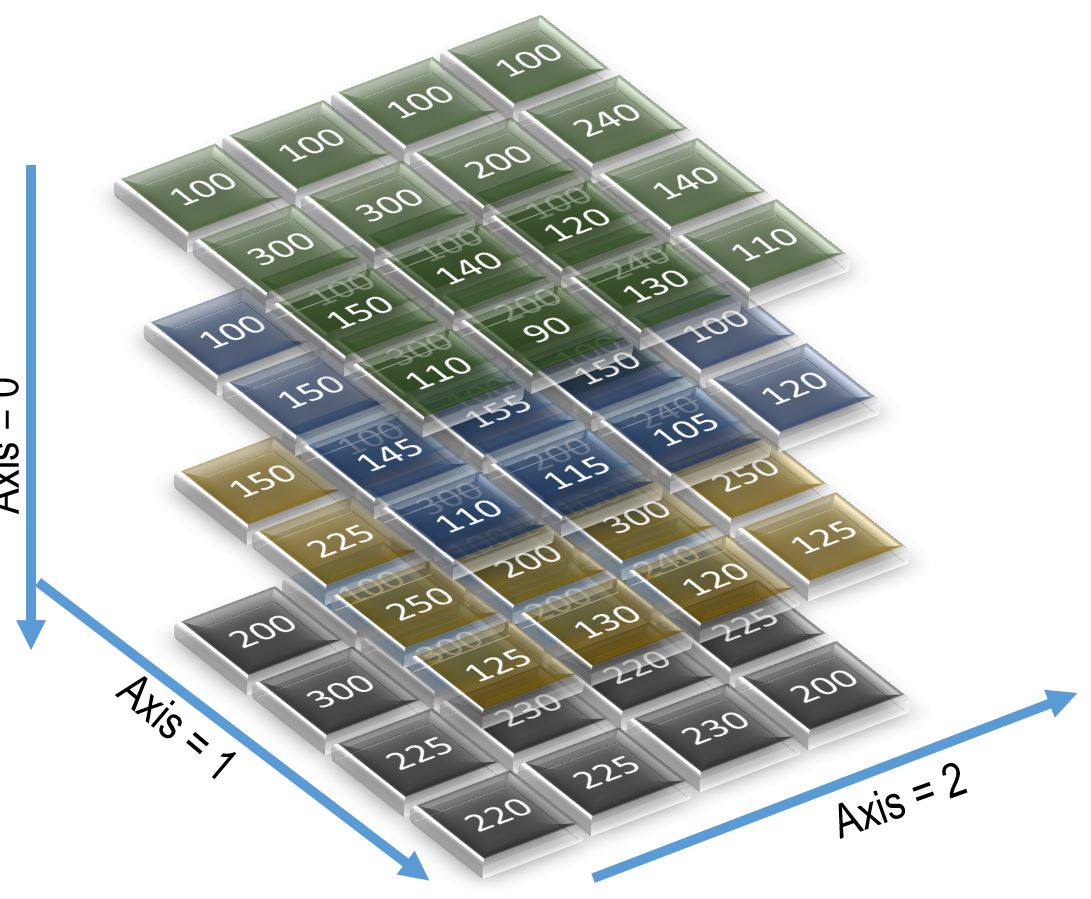
Figure 1. The 3-D sales array
The axes allow us to easily summarize the data contained in the cells on the respective axes. Take, for instance, a situation in which we want to know the sum of all sales for all products across all quarters. Note that we don't want the sum of all sales, which will give us just one number. We also don't want to know the sum of the sales of each product. We want the total sales of each product for each quarter; that is, we want a 2-D array. The dimensions are product and quarter. To do this, we will need to compute the sum of all numbers along axis=0. Figure 2 shows how one cell of the resultant 2-D array is calculated along axis=0. All the red-marked cells are summed to come to the number 550.
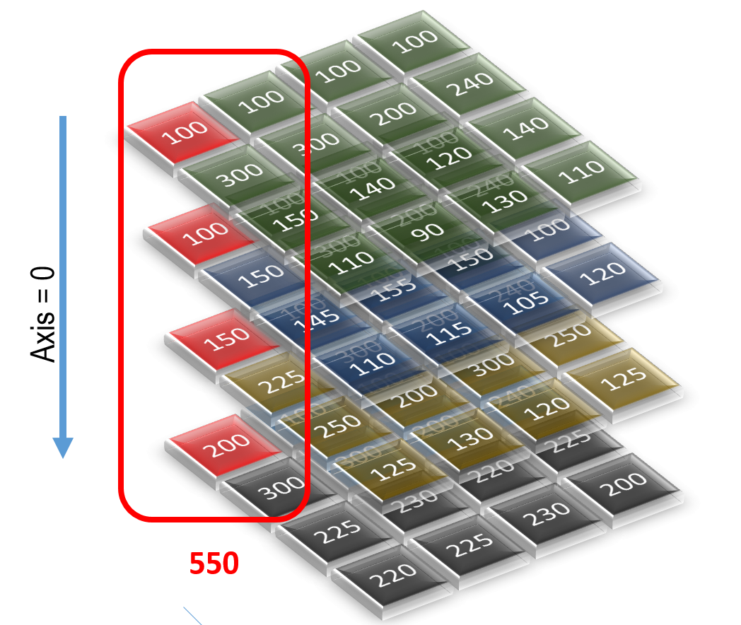
Figure 2. Calculation along axis=0
Likewise, all the other cells are summed in the same manner. Here is the result when we sum the array along axis=0.
>>> sales.sum(axis=0)
array([[ 550, 580, 520, 550],
   \[ 975, 1030,  810,  935\],

   \[ 770,  725,  790,  715\],

   \[ 565,  560,  585,  555\]\])
But the power of array summarization is way more than this. What if we wanted to find the sum of sales for all quarters, not products? It will also be a 2-D array; but the dimensions will not be product and quarter. They will be quarter and territory. This will be summed along axis=1, as shown in Figure 3. The total of one such set of cells comes to 660. Likewise Python computes the rest of the sets of cells and produces the results. Here is how the final calculated values look.
>>> sales.sum(axis=1)
array([[ 660, 630, 550, 590],
   \[ 505,  520,  495,  490\],

   \[ 750,  690,  810,  750\],

   \[ 945, 1055,  850,  925\]\])
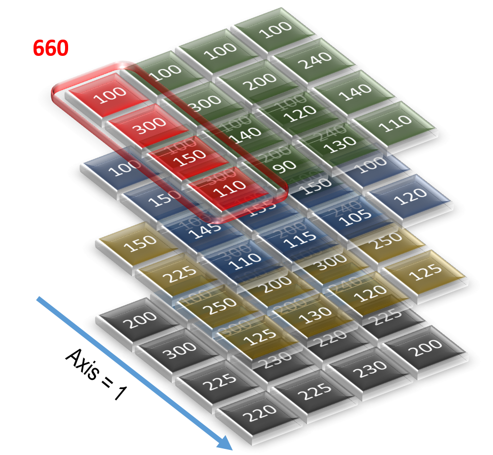
Figure 3. Finding the sum of sales for all quarters
Similarly, what if we wanted to find the total sales for products and territories, summed for all quarters? We can do that by computing the sum along axis=2. Figure 4 shows the calculation of one set of cells. The total comes out to be 400. Likewise, Python computes the sums for all cells and populates the 2-D array. Here is how we get the sum of all sales along axis=2.
>>> sales.sum(axis=2)
array([[ 400, 1040, 550, 440],
   \[ 400,  610,  550,  450\],

   \[ 600,  900, 1000,  500\],

   \[ 800, 1200,  900,  875\]\])
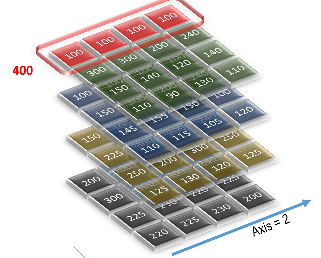
Figure 4. Finding the total of sales for all products and territories, summed for all quarters
I used the sum() function merely to demonstrate the effect of the summarization of this 3-D array along individual axes. You can use a lot more. For instance, if you wanted to find out the minimum sales amount of products for each quarter, you could have used this:
>>> sales.min(axis=0)
array([[100, 90, 100, 100],
   \[150, 160, 130, 170\],

   \[145, 140, 120, 100\],

   \[110,  90, 105, 110\]\])
Some other functions are mean() and max().
Each child array of the NumPy array can be addressed individually, as shown below:
>>> for row in sales:
... print (row)
[[100 90 100 100]
[150 160 130 170]
[145 140 120 100]
[110 90 105 110]]
[[100 100 110 100]
[225 220 200 225]
...
This function returns the output in an array form, which is useful if you want to operate on arrays as well. If you want to operate on individual elements of the array, you need to "flatten" it using the flat() function, as shown below:
>>> for sales_point in sales.flat:
... print(sales_point)
100
90
...
I hope you see how NumPy is useful for data analysis. Of course, it is not possible to show the complete power of the module in this short article. My intention was to give you a glimpse into the basics of NumPy and what possibilities it offers for data professionals. I encourage you to explore more of NumPy in the official NumPy documentation. Later in this article, you will also see some advanced uses of NumPy, especially integrating with other modules.
MatPlotLib
As they say, a picture is worth thousand words. It can't be more true for a data professional. Volumes of data are facts; but they are not necessarily the knowledge that you seek. Creating a graph or a chart of the data may show exactly what you want. Typically you probably put the data in a CSV file, export into a spreadsheet application such as MS Excel or your favorite data analysis application such as Tableau, and create the charts. Well, that is not exactly convenient. The process has many steps, leading to latency in the development of the charts and, therefore, reducing their effectiveness. It also forces you to perform an intermediate step of dumping data into a file for further analysis. Because you are using Python, you would want to complete everything in that environment without an intermediate step. Besides saving time, that also allows you to script the steps so that the process of going from data analysis to chart presentation can be automated. But how do you create a chart in Python from the data?
This is where the next module we will discuss becomes extremely handy. It's called MatPlotLib, and it's used to draw various types of charts to render data visually. Install the module first, as shown at the beginning of the article. You should also have installed NumPy, which was explained in the previous section.
Let's see the tool in action. First, we will need to import the modules into our environment. Instead of importing the entire MatPlotLib, we will import only the chart plotting functionality from it. We will also use aliases for these modules to save some typing.
>>> import numpy as np
>>> import matplotlib.pyplot as plt
We will use the data from the previous section where we defined a three-dimensional sales array. Let me define that again:
sales = np.array([
\[

    \[50,50,50,50\],

    \[150,150,180,120\],

    \[75,70,60,70\],

    \[55,45,65,55\]

\],

\[

    \[100,90,110,100\],

    \[150,160,130,170\],

    \[145,155,150,100\],

    \[110,115,105,120\]

\],

\[

    \[150,140,160,150\],

    \[225,220,230,225\],

    \[250,200,300,250\],

    \[125,130,120,125\]

\],

\[

    \[200,250,150,200\],

    \[300,350,250,300\],

    \[225,230,220,225\],

    \[220,225,230,200\]

\]

\])
We will use the simplest charts of all—line graphs of sales of products for each territory for the first quarter. On the x-axis, we just need a series of four numbers to represent the territories. So we define a variable—named simply x—to hold this array.
>>> x = np.array([0, 1, 2, 3])
On the y-axis, however, we need four variables—one for each product. Let's define one array variable for each product. Each of these variables—y0, y1, y2, and y3—will be an array.
>>> y0 = sales[0][0]
>>> y1 = sales[0][1]
>>> y2 = sales[0][2]
>>> y3 = sales[0][3]
Then we will plot a chart of the x and y values. We can optionally add a label. That's useful here because there will be four lines, and we will need to know what is for what:
>>> plt.plot(x,y0,label='Product 0')
[<matplotlib.lines.Line2D object at 0x03370CB0>]
>>> plt.plot(x,y1,label='Product 1')
[<matplotlib.lines.Line2D object at 0x03370D90>]
>>> plt.plot(x,y2,label='Product 2')
[<matplotlib.lines.Line2D object at 0x03375710>]
>>> plt.plot(x,y3,label='Product 3')
[<matplotlib.lines.Line2D object at 0x03375BB0>]
The legend describing the labels might come up on the chart at an inconvenient location. So, as an optional step, we can tell MatPlotLib to put the legend in a specific location, for example, the upper left corner:
>>> plt.legend(loc='upper left')
Finally, we tell MatPlotLib to show the chart:
>>> plt.show()
And voila! This will bring up a chart shown in Figure 5. The important thing to note is that you didn't need to have any special software installed to show the graph. It comes up in a different window.
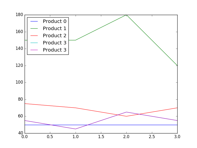
Figure 5. Chart generated by MatPlotLib
What if you wanted to show the data as a bar chart instead of lines? No worries. The bar() function is for that purpose. Use it instead of the plot() function used in the previous code. In addition to the other parameters you saw earlier, we will use a new parameter, color, to show what color the individual items will be displayed in. The color attribute is available in line chart as well.
plt.bar(x,y0,label='Product 0', color='blue')
plt.bar(x,y1,label='Product 1', color='red')
plt.bar(x,y2,label='Product 2', color='green')
plt.bar(x,y3,label='Product 3', color='yellow')
plt.legend(loc='upper left')plt.show()
The code above will bring up a bar chart (not shown). You will notice come controls on the chart window to zoom in (or out) on the chart to show the details. You can also save the chart as a picture by clicking the appropriate button. That is how I saved the image shown in Figure 5.
Like NumPy, this is merely a basic treatise on the MatPlotLib module. It can do many other things, especially 3-D graphs, which are not discussed here due to lack of space. I encourage you to explore the documentation, especially that of pyplot. In the next section, we will use NumPy and MatPlotLib to build something more powerful for data analysis.
Pandas
While NumPy provides many powerful data manipulation functionalities, it might not be as powerful as needed in some cases. That's were a new module—built on the top of NumPy—comes in. It's called Pandas. You have to install the module, as described at the beginning of the article. Once installed, you have to import it into your Python session. Below, we import all the modules we learned about so far:
>>> import pandas as pd
>>> import numpy as np
>>> import matplotlib.pyplot as plt
Pandas provides two types of collections for data analysis:
- Series, which is just a one-dimensional array
- DataFrame, which is two-dimensional array
Let's examine a simple series. In the earlier sections, we created a NumPy array to store the sales figure of the company for all products with a detailed breakdown for all quarters and all the four territories or zones. However, we didn't actually name the zones as North, South, and so on. Instead we just used their positional indices (0, 1, and so on). Ideally you would like to represent the data in a tabular format in the same way it is shown in table, with proper labels identifying the names of the axes such as this:
| | Prod 1 | Prod 2 | Prod 3 | Prod 4 |
| North | | | | |
| South | | | | |
| East | | | | |
| West | | | | |
First, we will create a series named zones to hold all the zone names. The Series (note the uppercase "S") function in the module Pandas creates the series.
>>> zones = pd.Series (['North','South','East','West'])
Let's take a look at the zones variable.
>>> zones
0 North
1 South
2 East
3 West
dtype: object
The products will be akin to the columns of a table; that is, they will be pretty much fixed. So we define a normal tuple named products. Below, only three products are used deliberately to contrast between the numbers of rows and columns.
>>> products = ('Prod 1','Prod 2','Prod 3')
Now that we have defined rows and columns, we need to enter the sales data. We can enter the data as a NumPy array, as we saw earlier. Let's examine a new concept. There is a built-in random number generator in NumPy. We can create a series of random numbers to store data. Because we need four rows and three columns, we will need to create a grid of that shape. The following command creates a set of random number arranged as four rows and three columns.
>>> data1 = np.random.randn(4,3)
Let's take a look at the variable named data1:
>>> data1
array([[-0.1700711 , 1.05886638, -0.29129644],
   \[ 1.5863526 , -1.10870921, -1.43207089\],

   \[ 0.74046798, -0.45139616,  0.90758052\],

   \[ 0.83318995, -0.44284258, -1.08616932\]\])
This gives us a perfect set of data to put into the empty two-dimensional array we showed earlier.
That brings up the next important topic—the two-dimensional array. In Pandas, it's known as a DataFrame. If you are familiar with R, you might remember this particular term from there. To create a DataFrame in Pandas, we need three things:
- The actual data. We already have it in the variable
data1.
- The label for columns. We have also defined that as the variable
products.
- The labels for the rows, which is called "index" in a Python DataFrame. We have the variable
zones for that.
Here is how we define the DataFrame:
>>> df1 = pd.DataFrame(data1,index=zones, columns=products)
Let's take a look at the DataFrame we just defined:
>>> df1
Prod 1 Prod 2 Prod 3
North -0.170071 1.058866 -0.291296
South 1.586353 -1.108709 -1.432071
East 0.740468 -0.451396 0.907581
West 0.833190 -0.442843 -1.086169
To address the specific elements, we need to have some type of Python datatype, preferably an array. To see the values, use the following:
>>> df1.values
array([[-0.1700711 , 1.05886638, -0.29129644],
   \[ 1.5863526 , -1.10870921, -1.43207089\],

   \[ 0.74046798, -0.45139616,  0.90758052\],

   \[ 0.83318995, -0.44284258, -1.08616932\]\])
Note how it comes back as a NumPy array, which makes it possible for it to be managed as a NumPy object. For instance, you can update all the elements to 10 times their original values using one command.
>>> df2 = df1 * 10
>>> df2
Prod 1 Prod 2 Prod 3
North -1.700711 10.588664 -2.912964
South 15.863526 -11.087092 -14.320709
East 7.404680 -4.513962 9.075805
West 8.331900 -4.428426 -10.861693
Now that the DataFrame is in place, let's perform some analysis. Here is an example of quick statistics on the data elements. It shows some basic statistical operations on the values, for example, the total count, mean, standard deviation, maximum, minimum, and so on.
>>> df1.describe()
Prod 1 Prod 2 Prod 3
count 4.000000 4.000000 4.000000
mean 0.747485 -0.236020 -0.475489
std 0.719491 0.917874 1.038394
min -0.170071 -1.108709 -1.432071
25% 0.512833 -0.615724 -1.172645
50% 0.786829 -0.447119 -0.688733
75% 1.021481 -0.067415 0.008423
max 1.586353 1.058866 0.907581
In this case, we showed products as columns. What if you want to see the territories as columns? You can easily do that using the T attribute (which stands for "transform"):
>>> df2 = df1.T
>>> df2
North South East West
Prod 1 -0.170071 1.586353 0.740468 0.833190
Prod 2 1.058866 -1.108709 -0.451396 -0.442843
Prod 3 -0.291296 -1.432071 0.907581 -1.086169
>>> df2.describe()
North South East West
count 3.000000 3.000000 3.000000 3.000000
mean 0.199166 -0.318143 0.398884 -0.231941
std 0.746985 1.657247 0.741090 0.976906
min -0.291296 -1.432071 -0.451396 -1.086169
25% -0.230684 -1.270390 0.144536 -0.764506
50% -0.170071 -1.108709 0.740468 -0.442843
75% 0.444398 0.238822 0.824024 0.195174
max 1.058866 1.586353 0.907581 0.833190
Sometimes it's difficult to show all the results on the screen. All you want to see might be the first few lines. Here is how you can display only the first two lines:
>>> df1.head(2)
Prod 1 Prod 2 Prod 3
North -0.170071 1.058866 -0.291296
South 1.586353 -1.108709 -1.432071
Or, the last two lines:
>>> df1.tail(2)
Prod 1 Prod 2 Prod 3
East 0.740468 -0.451396 0.907581
West 0.833190 -0.442843 -1.086169
In Pandas, the columns are called, well, "columns." The rows are called "rows." The labels for the rows are called "indexes." To see the labels for the DataFrame, display the index attribute:
>>> df1.index
Index(['North', 'South', 'East', 'West'], dtype='object')
To display the columns, do this:
>>> df1.columns
Index(['Prod 1', 'Prod 2', 'Prod 3'], dtype='object')
Sorting
What if you want to display the values in a sorted manner, instead of the way in which they were put in, to see how the values progress—much like how you would have done in a spreadsheet application? It's quite simple, using the sort_values() function. Here is the actual DataFrame called df1:
>>> df1
Prod 1 Prod 2 Prod 3
North -0.170071 1.058866 -0.291296
South 1.586353 -1.108709 -1.432071
East 0.740468 -0.451396 0.907581
West 0.833190 -0.442843 -1.086169
To sort it along the column called "Prod 1," you call the function with that column as a parameter:
>>> df1.sort_values('Prod 1')