Data Warehousing with Oracle Data Integrator 12cR2

Learn the basics of data warehouse development using Oracle Data Integrator 12cR2.

By Yuli Vasiliev

Oracle Data Integrator 12c (12.2.1.1) introduces support for dimensional objects: cubes and dimensions, which you can now create and edit using predefined forms available from the Designer Navigator in ODI Studio. In prior releases, to build a dimensional model, you had to directly operate on the underlying tables representing dimensional objects. Starting with release 12.2.1.1, you don't have to go down to the physical implementation when defining a dimensional object, manipulating its underlying structures directly. In contrast, all the definitions for a dimensional object can be created and modified through its multi-tab panel in ODI Studio, while the physical implementation is maintained for you implicitly.

This article illustrates how you can access this new functionality when implementing a typical Data Warehousing project in ODI Studio.

Planning the Sample Data Warehousing Project

It is fairly obvious that planning is the first thing to do when it comes to a new project. In case of a data-warehousing project, you have to decide on dimensional objects to be used and their structure as well as on data sources to populate those dimensional objects.

Starting with a scenario for the article sample, suppose you need to develop a simple data warehouse through a dimensional model in ODI Studio. Say, you have thousands of PO documents that you want to load into a data warehouse for analysis purposes. For the purpose of the article sample, you can use the PurchaseOrders.dmp dump file that contains 10,000 sample PO documents in JSON format. This files comes with Oracle Database 12c as a sample data source and can be found at $ORACLE_HOME/demo/schema/order_entry on each computer where Oracle Database 12c is installed.

In fact, a typical data warehouse usually includes at least one cube and several dimensions associated with it. However, since the main focus of this article is the new dimensional object support available in ODI 12cR2, it will take you through creating a single cube and a single dimension associated with it, showing this new functionality in action

As far as a dataset of PO documents is concerned, a cube you can build on top if it is going to be a Sales cube one way or another, typically including dollar amount as a measure. Although a typical Sales cube may contain multiple measures, the cube in this sample will have, for simplicity, a single measure: Amount. The other thing each cube must have are dimensions, which form its edges. As stated above however, this sample cube will have a single dimension – just to demonstrate how a dimension can be defined in ODI 12.2.1.1 or later.

To figure out which dimension will serve demonstration purposes in the best way for this sample, it would be useful to take a closer look at the PO documents in PurchaseOrders.dmp that will be used as the data source. So, drilling down on the sample PO structure, you may notice that it doesn’t contain enough information needed to create, for example, a three-level Product dimension, because products included in POs are not even categorized into groups. As for customers, they are not specified in POs at all, but only their addresses, which by the way contain enough information to define a Geography dimension with the following hierarchy: Total > Country > City.

Note: In a real project, the decision on dimensions and their structure naturally comes from the business questions you need to get answered, which, in turn, come from the business goals your project must meet. In fact, using dimensions simplifies the process of deriving information from a data warehouse, since users can query it along known hierarchies. For this same reason, using dimensions improves query performance.

In summary, the dimensional model of the sample will include the following objects:

• Data source: PurchaseOrders.dmp
• Cube: Sales
• Dimension: Geography

When represented diagrammatically, the sample data warehouse might look as follows:

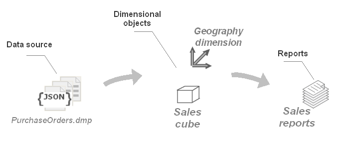
Figure 1: A high-level depiction of the sample data warehouse application.

The arrows in the diagram show the flow of the sample data on its way to turning into meaningful information. Derived from the source, the data is loaded into the dimensional objects, which can be then queried for sales analysis and reporting. Of course, what you can see on the above diagram is a high-level depiction: it doesn’t show the object structure, nor does it show the underlying objects and their relationships.

General Implementation Steps in ODI Studio

Now that you know where to go, you need to work out how to get there with ODI Studio. This section outlines only general steps, while the details are provided in the subsequent sections.

Listed as short bullets, here are the tasks you need to complete in ODI Studio to implement the article sample:

• Creating an ODI model for the data source
• Creating the underlying tables for the dimensional objects
• Creating the Geography dimension
• Creating the Sales cube
• Creating a mapping to load the Geography dimension
• Creating a mapping to load the Sales cube

As you might guess, most of the work should be done inside ODI Studio and only creating the underlying tables for the dimensional objects can be done in the underlying database directly.

Preparing Your Working Environment

Before proceeding to the implementation, make sure you have all the necessary software components installed on your computer. In particular, you’ll need the following two products installed in your system in order to follow the sample provided in this article:

• Oracle Database 12c (or above)
• Oracle Data Integrator 12cR2 (12.2.1.1.0) (or above)

If you don’t have them already installed, the quickest way to get started is to take advantage of the pre-built virtual machine for Oracle Data Integrator 12c that you can run within Oracle VM VirtualBox. An installation of Oracle VM VirtualBox takes just a few minutes. The list of supported operating system currently includes Windows, Mac OS X, Linux and Oracle Solaris. Once you have Oracle VM VirtualBox installed, you can download and then import the Oracle Data Integrator 12c VM appliance into it.

Once you have Oracle Data Integrator 12cR2 installed, make sure to create and configure ODI Master repository and Work repository. In the case of the Oracle Data Integrator 12c VM for Oracle VM VirtualBox mentioned above, you can skip this step, since the ODI installation includes these repositories pre-installed. Otherwise, refer to the Oracle® Fusion Middleware documentation, which describes this process in detail: section Creating the Master and Work Repository Schemas of the Installing and Configuring Oracle Data Integrator manual.

Creating a New Repository Connection (Optional)

The Oracle Data Integrator 12c installation in the VM mentioned in the previous section comes with a number of predefined repository connections, each of which is associated with a demonstration project. You can optionally create a new repository connection to use for the project you will create in this article.

So, to create a new repository connection, click the New button in the Oracle Data Integrator Login dialog, which appears once you’ve entered the password in the Wallet Password dialog when connecting to the repository. As a result, you should see the Repository Connection Information dialog that you need to fill in as follows (in case of the VM mentioned above, the password for the SUPERVISOR user is set to SUPERVISOR, and the password for the prod_odi_repo user is set to oracle). Also, make sure to specify actual database connection parameters in the URL field:

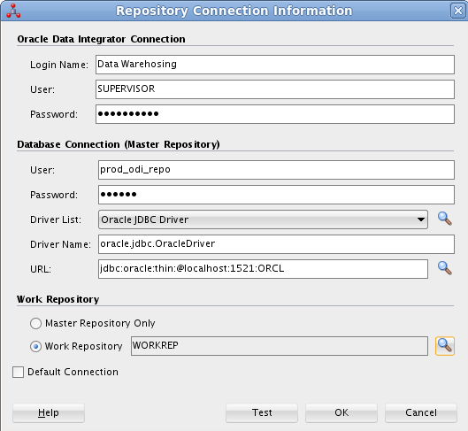
Figure 2: Creating a new repository connection.

Before you click OK to save the information for the newly created connection, you can click Test to make sure the connection is successful.

Creating an ODI Model for the Data Source

As mentioned, the PurchaseOrders.dmp dump file will be used as a data source to load the sample data warehouse. I covered the process of creating an ODI model for PurchaseOrders.dmp in my preceding OTN article: Constructing a Dimensional Environment with Oracle Database and ODI 12c. For detailed steps, see section Including JSON as a Source in ODI 12c in that article.

This section provides general steps, detailing only the most challenging parts of the process.

So what you need to do in general steps:

• Set up a topology for Complex File:
  • Define a physical schema for PurchaseOrders.dmp
  • Define a logical schema on top of the above physical schema
• Define a model based on the above topology

As you can see, before you can define a model, you must create a topology for it. In this particular case, you need to set up a topology for Complex File (since PurchaseOrder.dmp contains data in JSON format, if you recall), defining a physical schema for PurchaseOrders.dmp followed by defining a logical schema on top of that physical schema.

The most challenging part is defining a physical schema for PurchaseOrders.dmp. One of the steps during this process is to create a native XSD (nXSD) schema for translation of the JSON data derived from PurchaseOrders.dmp. You can easily do it with the help of the Native Format Builder wizard. The tricky part is that the wizard requires a single JSON document to generate an nXSD file, while PurchaseOrders.dmp includes 10,000. So, you’ll need to create a separate file with a single PO within to provide the wizard with. Since all the POs in PurchaseOrders.dmp are structurally identical, you can choose any one for that. Before doing this however, you need to fix something in PurchaseOrders.dmp.

Looking carefully at the JSON structure of a PO, you may notice that the names of some of the objects in the document are composed of two words, for example: ShippingInstructions and Special Instructions. As you can see, the first one is written together, while the latter includes a separation gap, which may cause a problem or an unexpected result when generating an nXSD schema.

Further examination of the document structure shows that Special Instructions is the only JSON object name containing a gap. So what you need to do is to remove the gap in all appearances of Special Instructions in PurchaseOrders.dmp. This can be easily accomplished with the help of the Replace tool in your text editor. Once you have fixed this problem, you can create a separate file, for example, OnePurchaseOrder.dmp, and then insert a PO document into it from PurchaseOrders.dmp – you can choose the first one, for example:

{"PONumber":1,"Reference":"MSULLIVA-20141102","Requestor":"Martha Sullivan","User":"MSULLIVA","CostCenter":"A50","ShippingInstructions":{"name":"Martha Sullivan","Address":{"street":"200 Sporting Green","city":"South San Francisco","state":"CA","zipCode":99236,"country":"United States of America"},"Phone":[{"type":"Office","number":"979-555-6598"}]},"SpecialInstructions":"Surface Mail","LineItems":[{"ItemNumber":1,"Part":{"Description":"Run Lola Run","UnitPrice":19.95,"UPCCode":43396040144},"Quantity":7.0},{"ItemNumber":2,"Part":{"Description":"Felicia's Journey","UnitPrice":19.95,"UPCCode":12236101345},"Quantity":1.0},{"ItemNumber":3,"Part":{"Description":"Lost and Found","UnitPrice":19.95,"UPCCode":85391756323},"Quantity":8.0},{"ItemNumber":4,"Part":{"Description":"Karaoke: Rock & Roll Hits of 80's & 90's 8","UnitPrice":19.95,"UPCCode":13023009592},"Quantity":8.0},{"ItemNumber":5,"Part":{"Description":"Theremin: An Electronic Odyssey","UnitPrice":19.95,"UPCCode":27616864451},"Quantity":8.0}]}

After that, you can launch the Native Format Builder wizard. On the JSON File Description screen of the wizard, browse your file system to find and select OnePurchaseOrder.dmp as a sample JSON file.

The next problem you'll have to deal with is that the UPCCode element in the nXSD document generated by the wizard is set to type xsd:integer by default, which is not appropriate here, since UPCCode values are too long for integer. So, you need to change it to xsd:long. The good news is that the wizard allows you to manually edit the generated nXSD.

After completing the wizard, you’ll be again on the JDBC tab of the data server panel, from which you launched the wizard. Here, you need to fix another problem, which is the dp_numeric_lenght property that specifies the size of all the numeric columns in the underlying relational database is set by default to 10. This is obviously not enough for storing UPCCode values. So, you’ll need to go down to the Properties section on the JDBC tab of the data server panel, turn off the default checking for dp_numeric_length, and manually set its value to 14 to be on the safe side.

After you’ve completed the physical schema, you’ll need to define a logical schema on top of it and then a model. These steps should be straightforward. As mentioned, the entire process is described in detail in section Including JSON as a Source in ODI 12c of the OTN article: Constructing a Dimensional Environment with Oracle Database and ODI 12c.

Just to recap, the last step in defining a model for the PurchaseOrders.dmp data source is to launch a reverse-engineering process, which should result in a number of datastores, including the following tables: ADDRESS, LINEITEMS, PART, PHONE, PORDERS, and SHIPPINGINSTRUCTIONS. The screenshot below shows a fragment of the Designer tab under Models in ODI Studio, where you can see the model populated with the datastores listed above.

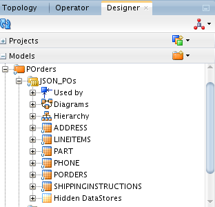
Figure 3: The model populated with the datastores reverse-engineered from PurchaseOrders.dmp.

What is clear from the above screenshot is that the JSON data derived from PurchaseOrders.dmp has been shredded into relational data and put into the tables generated as a result of a PurchaseOrders.dmp’s reverse engineering.

Creating the Underlying Tables for the Dimensional Objects

Now that you have the sample POs decomposed and stored as relational data, you can go ahead and create the dimensional objects that will be populated with that data. And the first step is to create the underlying tables for those objects. As stated earlier, you can create underlying tables directly in the database, using tools such as Oracle SQL Developer or SQLPlus:

1. Launch SQL Developer or SQLPLUS, and connect to the underlying database using an account with DBA privileges.
2. Create the DW1_PR schema and grant necessary privileges, by issuing the following commands:
   

   CREATE USER DW1_PR IDENTIFIED BY pswd;  GRANT CONNECT, RESOURCE TO DW1_PR;

3. Connect as DW1_PR, and create the geography_dm table, as well as the staging tables for the Geography dimension levels, as follows:
   

   CREATE TABLE dw1_pr.geography_dm( 
     DIMENSION_KEY  NUMBER, 
     TOTAL_SURROGATE_KEY NUMBER,   
     TOTAL_NATURAL_KEY VARCHAR2(30),
     TOTAL_NAME VARCHAR2(50), 
     COUNTRY_SURROGATE_KEY NUMBER,
     COUNTRY_NATURAL_KEY VARCHAR2(30), 
     COUNTRY_NAME VARCHAR2(50),
     CITY_SURROGATE_KEY NUMBER,
     CITY_NATURAL_KEY VARCHAR2(30), 
     CITY_NAME VARCHAR2(50), 
     CONSTRAINT geography_dm__pk PRIMARY KEY(DIMENSION_KEY)
   ); 
   
   CREATE TABLE dw1_pr.geography_city_stg(    
     DIMENSION_KEY  NUMBER, 
     TOTAL_SURROGATE_KEY NUMBER,
     TOTAL_NATURAL_KEY VARCHAR2(30), 
     TOTAL_NAME VARCHAR2(50), 
     COUNTRY_SURROGATE_KEY NUMBER, 
     COUNTRY_NATURAL_KEY VARCHAR2(30),
     COUNTRY_NAME VARCHAR2(50),
     CITY_SURROGATE_KEY NUMBER,
     CITY_NATURAL_KEY VARCHAR2(30), 
     CITY_NAME VARCHAR2(50)
   ); 
   
   CREATE TABLE dw1_pr.geography_country_stg(
     DIMENSION_KEY  NUMBER,
     TOTAL_SURROGATE_KEY NUMBER,
     TOTAL_NATURAL_KEY VARCHAR2(30),
     TOTAL_NAME VARCHAR2(50),
     COUNTRY_SURROGATE_KEY NUMBER,
     COUNTRY_NATURAL_KEY VARCHAR2(30),
     COUNTRY_NAME VARCHAR2(50)
   );
   
   CREATE TABLE dw1_pr.geography_total_stg(
     DIMENSION_KEY  NUMBER, 
     TOTAL_SURROGATE_KEY NUMBER,
     TOTAL_NATURAL_KEY VARCHAR2(30),
     TOTAL_NAME VARCHAR2(50)
   );

4. There is one more underlying database object you need to create for the Geography dimension. This is a sequence that will be used to generate surrogate key values. You can create it as follows:
   

   CREATE SEQUENCE geography_sq;

5. Then, create the sales_tab table with the following statement:
   

   CREATE TABLE dw1_pr.sales_tab(
       AMOUNT NUMBER(10,2), 
       QUANTITY NUMBER,
       COST NUMBER(10,2),
       GEOGRAPHY VARCHAR(50)
    );

    

   Before you can define dimensional objects on top of the above tables in ODI Studio, you must first reverse engineer these tables into an ODI model. As usual, creating a model comes after setting up a topology for it. The following steps will walk you through the entire process:

    

   The fist task is to define a data server corresponding to the DW1_PR schema in the underlying database:

    

6. On the Topology tab of ODI Studio, expand the Physical Architecture->Technologies node, and right-click Oracle. Then, select New Data Server.
7. On the Definition tab of the Data Server panel, enter the name for the data server you’re creating; for example: po_target. Then, enter orcl in the Instance / dblink (Data Server) field.
8. In the Connection section on the same tab, enter DW1_PR in the User field, and the actual password for this user in the Password field.
9. Move on to the JDBC tab of the Data Server panel. Select Oracle JDBC Driver in the JDBC Driver pull-down, and then enter the JDBC URL in the JDBC URL field, which might look like this: jdbc:oracle:thin:@localhost:1521:orcl
10. In the File menu of ODI Studio, select Save to save the data server you just defined.
11. Return to the Data Server panel, find and click the Test Connection button to verify connection.

     

    The next task in defining the topology is to create a physical schema for the data server defined above:

     

    On the Topology tab of ODI Studio, under the Physical Architecture->Technologies->Oracle node, right-click the newly created po_target, and select New Physical Schema.

     

12. On the Definition tab of the po_target.Schema panel, in Schema(Schema) select DW1_PR from the drop-down list. Then, select the same schema in Schema(Work Schema).
13. In the File menu of ODI Studio, select Save to save the physical schema.

     

    Then, you need to create a logical schema and associate it with the above physical schema:

     

14. the Topology tab of ODI Studio, expand the Logical Architecture->Technologies node, right-click Oracle, and then select New Logical Schema.
15. On the Definition tab in the Logical Schema panel, enter a name; for example: POrders_tgt. From the drop-down list under Physical Schemas, select the physical schema created in these steps earlier: po_target.DW1_PR.
16. In the File menu of ODI Studio, select Save to save the logical schema just created.

     

    Now you can create a model for the topology just defined:

     

17. On the Designer tab of ODI Studio, expand Models and right-click the POrders folder you should have already created. From the pop-up menu, select New Model.
18. On the Definition tab of the Model panel, enter a name in the Name field; for example, PO_TGT. Then, choose Oracle in the Technology pull-down, and POrders_tgt in the Logical Schema pull-down.

     

    Finally, you can reverse-engineer the model:

     

19. On the Reverse Engineer tab of the Model panel, click the Reverse Engineer button to launch a reverse-engineering process. Once it is completed, the following datastores: GEOGRAPHY_DM, GEOGRAPHY_TOTAL_STG, GEOGRAPHY_COUNTRY_STG, GEOGRAPHY_CITY_STG, and SALES_TAB should appear under the POrders->PO_TGT node within the Models panel, as shown in the screenshot below.

     

    

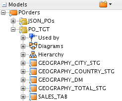
Figure 4: The model reverse-engineered from the underlying database.

Having the underlying tables created and reverse-engineered into an ODI model, you can move on to the task of defining dimensional objects on top of those tables.

Defining a Sequence in ODI Studio

Before proceeding to the task of defining the Geography dimension however, there is still one more underlying object to be defined in advance. This is a sequence that will be used to automatically generate surrogate key values in the dimension table. In the previous section, you created sequence GEOGRAPHY_SQ in the underlying database. Now you need to make it available within ODI Studio.

In ODI Studio, you can define either a global sequence that can be then used in all projects or a project sequence limited to the project in which it is defined. Let’s choose the latter, creating first the project:

1. In the Designer tab, click the New Project button on the right of the Projects node, select New Project in the popup menu.
2. On the Project panel, in the Name field enter a project name; for example, DW1_PR.
3. In the File menu of ODI Studio menu, select Save to save the project.
4. On the Designer tab, expand the Projects->DW1_PR node, right-click Sequences, and select New Sequence from the popup menu.
5. In the new sequence creation form, enter GEOGRAPHY_SQ in the Name field and leave 1 in the Increment field. Then, go down to the Sequence configuration section, select Native sequence and choose POrders_tgt from the Schema drop-down list. Then, click the magnifying glass on the right of the Native sequence name field.
6. In the Native sequence choice dialog, choose CLOBAL from the Context drop-down list, then select GEOGRAPHY_SQ from the Select the native sequence to use list, click OK.
7. In the File menu of ODI Studio, select Save to save the newly created sequence.

By now, you have all the necessary components to define the Geography dimension. Read on to learn how.

Defining the Geography Dimension

As mentioned, for the sake of simplicity the sales data set used in this sample has a single dimension: Geography, which has a three-level hierarchy: Total > Country > City.

The following steps will walk you through the process of defining the Geography dimension in ODI Studio:

1. On the Designer tab of ODI Studio, click the New Dimensional Model button on the right of Dimensions and Cubes node, and select New Dimensional Model.
2. On the Definition tab of the New Dimensional Model panel, enter DW1 as the name for the dimensional model you're creating.
3. In the File menu of ODI Studio menu, select Save to make the newly created dimensional model available under the Dimensions and Cubes node.
4. Under Dimensions and Cubes expand DW1, right-click Dimensions and select New Dimension.
5. On the Definition tab of the new dimension panel, enter Geography as the name for the dimension being created. Move on to the Binding section and click the magnifying glass to the right of the Datastore field.
6. In the Select Datastore dialog, select the GEOGRAPHY_DM datastore that you'll find under the POrders->PO_TGT model folder. Click OK.

    

   

    

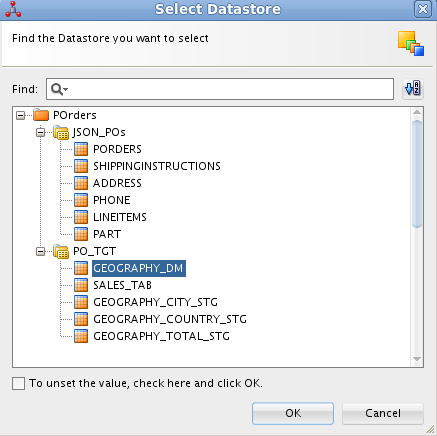
   Figure 5: Selecting the datastore for the dimension being created.

7. Then, click the magnifying glass to the right of the Surrogate Key Sequence field and browse for the GEOGRAPHY_SQ sequence. After that, the Geography dimension panel should look as shown in the screenshot below:

    

   

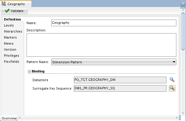
   Figure 6: The Definition tab of the Geography dimension.

    

8. In the File menu of ODI Studio, select Save to save the Geography dimension.

    

   Defining a dimension, you specify its levels and hierarchies. For the Geography dimension discussed here, this can be done as follows:

    

9. In the Geography dimension panel, move on to the Levels tab.

    

   Start with defining the Total level:

    

10. In the Levels table, click the Add button. In the newly created level row, change the name from LEVEL1 to Total. The Datastore field should be automatically filled in with PO_TGT.GEOGRAPHY_DM. In the Staging Datastore field, click the … button (in the right corner).
11. the Select Datastore dialog, select the GEOGRAPHY_TOTAL_STG datastore that you'll find under the POrders->PO_TGT model folder, click OK.
12. Move down to the Level Attributes table, and click the Select Columns... button in the table menu bar. Make sure to check only the following columns:
    • Name
    • Surrogate Key
    • Data Type
    • Size
    • Attribute
    • Staging Attribute
13. In the Level Attributes table menu bar, click the Add button to add a new attribute for the Total level. You'll need to repeat it two more times, entering or selecting the values as shown below:

     

    

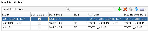
    Figure 7: Level attributes for the Total level.

     

14. Scroll down to the Natural Key Members table, and click Add. As a result, you should see the NATURAL_KEY row added to the table.

     

    Then, define the Country level:

     

15. Return  to the Levels table, and click Add. In the generated row, change the name from LEVEL1 to Country. Once again, the Datastore field should be automatically filled in with PO_TGT.GEOGRAPHY_DM. In the Staging Datastore field, click the … button (in the right corner).
16. In the Select Datastore dialog, select the GEOGRAPHY_COUNTRY_STG datastore under the POrders->PO_TGT model folder, and click OK.
17. In the Level Attributes table, add three level attributes for the Country level, setting up the values as shown below:

     

    

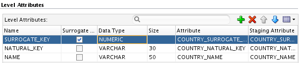
    Figure 8: Level attributes for the Country level.

     

18. In the Natural Key Members table, click Add to add the NATURAL_KEY level attribute.
19. Scroll down to the Parent Level References section, and click the Add button from the Parent References table button panel. In the generated row, change the name from PARENTREF1 to Country_of_Total. In the Parent Level field, select Total. Also make sure the Parent Level Reference Key Member table below shows the row with the Parent Key Attribute field set to GEOGRAPHY_DM.TOTAL_SURROGATE_KEY, the Foreign Key Attribute field set to TOTAL_SURROGATE_KEY, and the Foreign Key Staging Attribute field is also set to TOTAL_SURROGATE_KEY, as shown in the figure below:

     

    

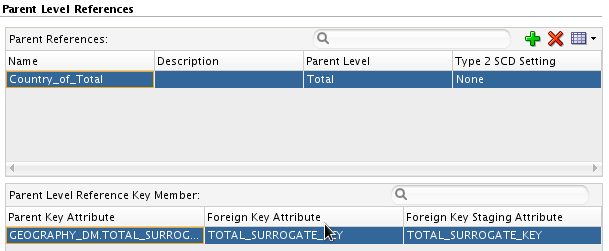
    Figure 9: Parent references for the Country level.

     

    Finally, define the City level

     

20. Return to the Levels table, and click Add. In the generated row, change the name from LEVEL1 to City. In the Staging Datastore field, click the … button (in the right corner).
21. In the Select Datastore dialog, select the GEOGRAPHY_CITY_STG datastore under the POrders->PO_TGT model folder, and click OK.
22. In the Level Attributes table, add three level attributes for the City level, setting up the values as shown below:

     

    

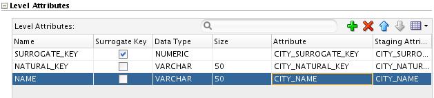
    Figure 10: Level attributes for the City level.

     

23. In the Natural Key Members table, click Add to add the NATURAL_KEY level attribute
24. In the Parent References table, click Add. In the generated row, change the name from PARENTREF1 to City_of_Country. In the Parent Level field, select Country. Then, make sure the Parent Level Reference Key Member table below shows the row with the Parent Key Attribute field set to GEOGRAPHY_DM.COUNTRY_SURROGATE_KEY, the Foreign Key Attribute field set to COUNTRY_SURROGATE_KEY, and the Foreign Key Staging Attribute field is also set to COUNTRY_SURROGATE_KEY.

     

    After defining the levels, you can move on to defining hierarchies.

     

25. Move on to the Hierarchies tab. In the Hierarchies table, click Add, change the name from HIERARCHY1 to CHEOGRAPHY_DEF_HIERARCHY, and turn on the Default checkbox.
26. In the Hierarchy Members, add the levels defined in the above steps, as shown in the screenshot below:

     

    

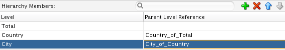
    Figure 11: Hierarchy members for the Geography default hierarchy.

27. In the top-left corner of the Geography dimension editor, click the Validate button. You should see the Successful validation popup window. Otherwise check out the Validation Results window.
28. In the File menu of ODI Studio, select Save.

This completes the process of defining the Geography dimension. In the Creating the Geography Dimension Load Mapping section later in this article, you'll look at how to map this dimension to the source and then populate with data.

Defining the Cube

Once the dimensions are defined, you can go ahead and define the cube whose edges are formed of those dimensions. What this means in this particular project is that you can proceed to defining the Sales cube once the Geography dimension has been defined.

The steps below walk you through the process of creating the Sales cube:

1. Under Dimensions and Cubes expand      newly created DW1, right-click Cubes and select New Cube.
2. On the Definition tab of the new      cube panel, enter Sales as the name for the cube. Move on to the Binding      section and click the magnifying glass to the right of the Datastore      field.
3. In the Select Datastore dialog,      select the SALES_TAB datastore that you'll find under the      POrders->PO_TGT model folder. Click OK.
4. In the File menu of ODI Studio,      select Save.
5. In the Sales cube panel, click the      Details tab.
6. In the Dimensions table, click      Add. Then, in the Level field, click the ... button.
7. In the Select Level dialog box,      select City.
8. In the Key Binding table, edit the      generated row, selecting GEOGRAPHY in the Attribute field.
9. Move down to the Measures table in      the Details page, click the Select Columns... button in the table menu      bar, and check only the following five columns:
   • Name
   • Data Type
   • Size
   • Scale
   • Attribute
10. Using the Add button in the      Measures table menu bar, add the following three measures for the cube:      AMOUNT, COST, and QUANTITY, entering or selecting the values illustrated      in the screenshot below:

     

    

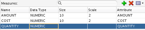
    Figure 12: Measures for the Sales cube.

11. In the top-left corner of the Sales cube editor, click the Validate button.
12. In the File menu of ODI Studio, select Save.

Now that you have defined the dimensional objects, the next step is to map them to their data sources.

Creating the Geography Dimension Load Mapping

This section describes how to create a mapping that is to load the Geography dimension defined in the Defining the Geography Dimension section earlier in this article. Before proceeding to the detailed steps, let's outline things to be done in general. So, below are the general steps you need to accomplish in order to implement the Geography Dimension Load mapping:

1. Create a mapping under the DW1_PR      project.
2. Drag and drop the Address table      and the Geography dimension into the mapping.
3. Drag and drop component EXPRESSION      from the Components palette into the mapping.
4. Create connections between      components on the mapping to define the data flow.

Now that you have an idea of what to be done, the following steps will walk you through the process in detail:

1. On the Designer tab, expand      Projects->DW1_PR->First Folder. Right-click Mappings and select New      Mapping in the popup menu.
2. In the New Mapping dialog, enter      Geography Dimension Load, and click OK.

    

   Looking through the relational tables reverse-engineered from the PurchaseOrders.dmp file, it's easy to guess that only the Address table may contain the data needed to populate the Geography dimension.

3. On the Designer tab, expand      Models->POrders->JSON_POs, then drag the ADDRESS table into the      mapping area.
4. On the Designer tab, expand      Dimensions and Cubes->DW1->Dimensions. Drag Geography into the      mapping area on the right of the Address table.
5. From the Components palette, drag      EXPRESSION into the mapping area, and drop it on the left side of      Geography that you should already have on the mapping. Move on to the      EXPRESSION - Properties pane. On the Attributes tab, click the Add      Attribute button on the Attributes table menu bar, and enter the following      attribute:

    

       Name: TOTAL_NAME

       Data Type: VARCHAR
         Length: 25
         Expression: 'Geography_Total'

6. In the mapping area, drag and drop EXPRESSION's TOTAL_NAME to Geography's Total_Natural_Key. Then, drag and drop EXPRESSION's TOTAL_NAME to Geography's Total_Name, so the mapping area should look now as follows:

    

   

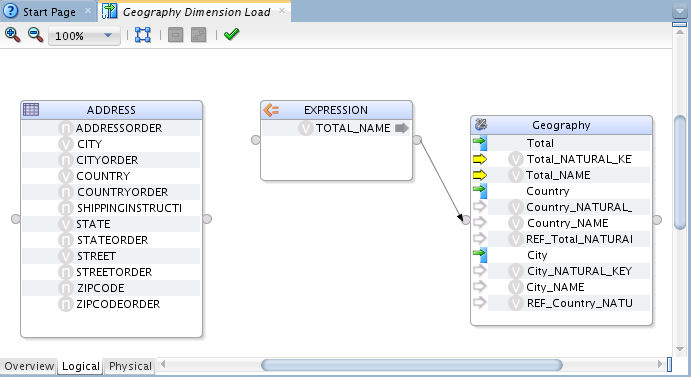
   Figure 13: Connecting the Expression component the Geography dimension.

    

7. Drag and drop Address' COUNTRY to      Geography's Country_Natural_Key, Geography's Country_Name, and Geography's      REF_Country_Natural_Key. Then, drag and drop Address' CITY to Geography's      City_Natural_Key and Geography's City_Name.
8. In the Geography dimension on the      mapping, select REF_Total_Natural_Key. Then, move on to the Properties      pane and enter 'Geography_Total' in the Expression field. The final design      for the Geography Dimension Load mapping should look as follows:

    

   

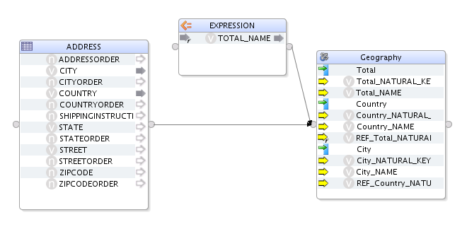
   Figure 14: Final design of the Geography Dimension Load mapping.

    

9. In the Diagram ODI menu bar, select Validate the Mapping. Then, in the File menu of ODI Studio, select Save.

The mapping you just created is ready to be executed to load the Geography dimension with the data. However, you can do it latter in a package along with the Sales Cube Load mapping that will be discussed in the next section.

Creating the Sales Cube Load Mapping

As you no doubt have realized, you won't be able to populate the Sales cube with a single dataset, as you did for the Geography dimension in the previous section. So, before proceeding to creating a mapping for loading the Sales cube, you'll need to spend some time examining the datasets to be used as the sources for populating the cube. Back to Figure 3 that shows the tables reverse-engineered from the PurchaseOrders.dmp file, take a closer look at PORDERS, LINEITEMS, PART, SHIPPINGINSTRUCTIONS, and ADDRESS, examining their relations. Thus, you may notice that tables ADDRESS and LINEITEMS can be joined to each other through the SHIPPINGINSTRUCTIONSFK and PORDERSFK attributes respectively, thus eliminating the need to use intermediary table PORDERS. But before that, you need to join tables LINEITEMS and PART using the following condition: LINEITEMS.LINEITEMSPK=PART.LINEITEMSFK.

The following steps take you through the entire process of creating the Sales Cube Load mapping:

1. On the Designer tab, expand      Projects->DW1_PR->First Folder. Right-click Mappings and select New      Mapping in the popup menu.
2. In the New Mapping dialog, enter      Sales Cube Load, and click OK.
3. On the Designer tab, expand      Models->POrders->JSON-POs, and then drag and drop LINEITEMS, PART,      and ADDRESS into the mapping area, one under the other.
4. From the Components palette, drag      JOIN into the mapping area, and drop it next to LINEITEMS and PART.
5. In the Mapping area, drag and drop      PART's LINEITEMSFK to JOIN, and drag and drop LINEITEMS's LINEITEMSPK to      JOIN.
6. In the JOIN - Properties pane, on      the Condition tab, enter LINEITEMS.LINEITEMSPK=PART.LINEITEMSFK in the      Join Condition field.
7. Repeat steps 4 through 6 to create      a join between the just created JOIN and ADDRESS, setting up      ADDRESS.SHIPPINGINSTRUCTIONSFK=LINEITEMS.PORDERSFK as the join      condition.
8. On the Designer tab, expand      Dimensions and Cubes->DW1->Cubes, and then drag the Sales cube into      the mapping area.
9. In the Mapping area, drag a link      between JOIN1 and Sales. As a result, the Attribute Matching dialog should      appear.
10. In the Attribute Matching dialog,      leave the matching options by default, click OK. Note that the mapping for      the Quantity attribute of the cube is done automatically, mapping      LINEITEMS.QUANTITY to Sales.Quantity.
11. Map the other attributes, as      follows:

    Finally, the mapping should look similar to the following screenshot:

     

    

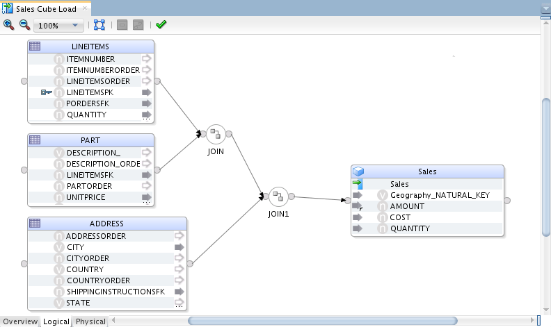
    Figure 15: Final design of the Sales Cube Load mapping.

    • ADDRESS.CITY to       SALES.Geography_NATURAL_KEY
    • PART.UNITPRICE*LINEITEMS.QUANTITY       to SALES.AMOUNT
    • PART.UNITPRICE to SALES.COST
12. In the Diagram menu of ODI Studio, select Validate the Mapping. Then, select Save from the File menu.

By now, you should have the Sales Cube Load mapping and the Geography Dimension Load mapping, both are ready for execution. The order of execution matters: the Geography Dimension Load mapping must be run first. In the following section, you’ll look at how to use the Packages feature in ODI to organize an execution of mappings in a predetermined order.

Execution the Mappings in a Package

In ODI Studio, you can take advantage of a package, which allows you to organize a sequence of execution steps into a diagram, so that each subsequent step is performed depending on the execution result of the preceding one (success or failure).

The following steps will walk you through the process of creating a package that will execute the Geography Dimension Load mapping and then, on success, will execute the Sales Cube Load mapping.

1. On the Designer tab, expand      Projects->DW1_PR->First Folder, right-click Packages and select New      Package.
2. In the New dialog, enter a name      for the package, for example Sales Cube Load, click OK.
3. On the Designer tab, expand      Projects->DW1_PR->First Folder->Mappings, drag and drop the      Geography Dimension Load mapping into the Sales Cube Load package diagram.
4. Drag and drop the Sales Cube Load      mapping into the Sales Cube Load package diagram, next to the Geography      Dimension Load mapping.
5. In the Package toolbar tab, click      the Next Step on Success button. Then, in the package diagram, drag a line      from Geography Dimension Load to Sales Cube Load:

    

   

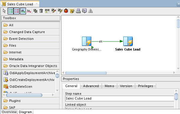
   Figure 16: Sales Cube Load package diagram.

6. In the File menu of ODI Studio,      select Save.
7. In the Run menu of ODI Studio, select Run. Then, click OK in the Run dialog to run the package.
8. Close the Session started window.

After completing the above steps, you will have dimensional objects: dimension Geography and cube Sales populated with the data derived from the PurchaseOrders.dmp data source. Physically, this means that underlying tables Geography_dm and Sales_tab have been populated with that data.

Conclusion

This article provided a detailed how-to on how you can take advantage of the cube and dimension creating and loading patterns, new functionality, available in Oracle Data Integrator 12c starting with release 12.2.1.1. Walking through the article sample, you looked at how using this new functionality can simplify the process of modeling and implementing a data warehouse.

See Also

• Oracle Data Integrator Documentation
• Oracle Data Integrator 12.2.1: Creating Cubes and Dimensions
• Introduction to Data Warehousing Concepts
• Constructing a Dimensional Environment with Oracle Database and ODI 12c
    Cube Development for Beginners

About the Author

Yuli Vasiliev is a software developer, freelance author, and consultant currently specializing in open source development, Java technologies, business intelligence (BI), databases, service-oriented architecture (SOA), and more recently virtualization. He is the author of a series of books on the Oracle technology, including Oracle Business Intelligence: An introduction to Business Analysis and Reporting (Packt) and PHP Oracle Web Development: Data processing, Security, Caching, XML, Web Services, and Ajax (Packt).